
Open Source TDCR Contact Model
In a previous blogpost, we explained a new approach for contact aided motion planning. As part of our OpenCR project, we have open sourced the model we use for simulation1. Additional implementation details and examples can be found in our paper2.
In this blog we present a tutorial on how to use our open source OpenTDCRContactModel. With our code, you can build custom taskspaces with circular obstacles and apply our contact-aided search to tendon driven continuum robots to reach a target position in a 2D taskspace. The model is implemented in C++ and Matlab. We also provide an easy to use interface written in Python. For a quickstart, have a look to our Google collab demo notebook.
Model Defintion
The model is posed as a nonlinear optimisation problem. The robot is said to be defined by ‘m’ piecewise constant curvature arcs. The objective of this problem is to find a set of m curvatures that minimize the robots potential energy. The nonlinear equality constraint makes sure that the input tendon length is equal to the calculated tendon length. The nonlinear inequality constraint ensures that points on the robot lie outside all the obstacles.
Code Organization
Installation instructions along with the source can be found here. The two important classes to know for this implementation is the Robot(radius, disk_num) class and Node(Robot, length, actuation) class. Node is used to describe the robot at some point in joint space. Node also has a method run_forward_model(taskspace, bool_reduced, model_type) which calculates the forward kinematics of the robot given its current joint space configuration. Two options are avaliable for model_type, model_type="KINEMATIC_MATLAB" or model_type="KINEMATIC_CPP". You can access the Node’s cartesian coordinates with Node.ee after calling run_forward_model.
The Robot class stores general configuration parameters of the robot like tendons, length and radius. Since the model uses a piece-wise constant curvature arc representation, the number of disks is used to discretize the backbone into that many subsegments. The robot object is then fed into each node object as a parameter.
Note: The robot lies in the xz plane and the model currently supports circular obstacles and 2d contact interactions.
Code Walkthrough
Taskspace
Obstacles in the taskspace are defined by the Circle(radius, (x, y, z)) class. More complex shapes can be formed by superimposing multiple circles.
Defining a taskspace is easy, just initialize a taskspace object then set each obstacle you want in your taskspace. Or alternatively, a default taskspace in /workspaces can be used.
workspace = TaskspaceCircle()
radius = 0.01
obstacle_1 = Circle(radius, (0.02, 0.0, 0.03))
obstacle_2 = Circle(radius, (-0.04, 0.0, 0.03))
obstacle_3 = Circle(radius, (0.08, 0.0, 0.03))
workspace.set_obstacles(obstacle_1, 1, 1)
workspace.set_obstacles(obstacle_2, 1, 1)
workspace.set_obstacles(obstacle_3, 1, 1)
The parameters for set_obstacles are,
# workspace.set_obstacles(Circle, n, z_delta)
#     Circle: new obstacle to add to the taskspace
#     n: add n copies offset by z_delta
#     z_delta: distance to offset the n copies
Robot
Once the taskspace is created, a TDCR Robot object is also created by specifying the radius and number of discrete disks composing the robot. A Node object is also created representing the robot at some configuration in time. In the starting position, the Node will be set to have 0.001 length and 0.001 actuation.
      # mod_cr.Robot(radius, disks)
robot = mod_cr.Robot(6e-3, 30)

            # Node(Robot, length, actuation)
config_init = Node(robot, 0.001, 0.001)
config_init.set_init_guess(np.array([1]*robot1.nd))
config_init.T = np.eye(4)

# Run First forward kinematic iteration
config_init.run_forward_model(workspace, True, "KINEMATIC_CPP")
Motion Planning
Next a motion plan must be created. A target location can be specified and the following method will generate a sequence of joint space values (tendon actuation and tendon length). This sequence will then be applied to the robot with forward kinematics to traverse it through the taskspace. Paths can be created using the following taskspace method. This method will save a generated path to a Nx2 csv file with each row being formatted as segment_length, tendon_length
taskspace.generate_path(initial_Node, target=[x, y, z], filename='filename')
This method performs a greedy heuristic search through joint space sequences using Euclidean distance as a metric. More details can be found in Rao et al.2 The heuristic can be replaced with a custom heuristic you wish to investigate. Feel free to play around with it. The heuristic is defined in /utils/taskspace.py. Alternatively, you may load one of the premade path located in /sample_paths.
Forward kinematics
After the path is created, we then iterate over each position in the joint space csv file previously created. The forward kinematics of each value is calculated and saved to a list traced_path.
prev_guess = config_init.var[0,::3]
sample_path = load_and_extract('sample_path.csv')
traced_path = [config_init]*len(sample_path)
for idx, iter in enumerate(sample_path):
    curr_node = Node(robot1, iter[0], iter[1])
    curr_node.set_init_guess(prev_guess)
    model_exitflag = curr_node.run_forward_model(workspace, True, "KINEMATIC_CPP")
    if model_exitflag:
        prev_guess = curr_node.var[0,::3]
        traced_path[idx] = curr_node
    else:
        print("Model did not converge")
        break
Selecting an Initial Guess:
The step on setting an initial guess with config_init.set_init_guess is important! As explained in the Model Definition section, the model used in our simulation environment is a complex nonlinear optimization problem. Additionally, the mapping between joint space and task space is not a one-to-one mapping during implicit contact motion. Setting a correct initial guess is crucial for model convergence. A rule of thumb that has worked well for us is to run the forward kinematics solver sequentially. This is done by setting the initial segment length and tendon length of the robot to be (0.001, 0.001) or as 1mm in units for each. Then the model slowly progresses in 1mm increments to remain stable. In each time step, the curvature values of the previous time frame is used as an initial guess for the next.
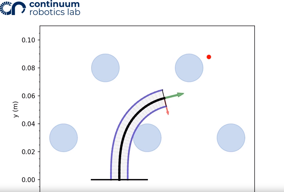
Visualizing a Configuration
After the model has been run, and the nodes curvature values are determined, we can visualize the robot and taskspace by plotting it. The red dot is our target position.
config_init.plot_configuration(workspace)
helpers.saveFigure()
# plt.show()
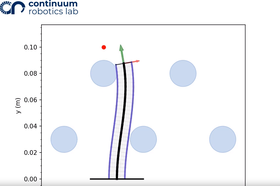
Visualizing a Motion Plan
For every motion plan that is generated and simulated, it can be visualized as a mp4 video.
helpers.visualizing(traced_path, workspace, "filename")
Using the default taskspace and 3_sample_path.csv, the resulting video is:
Happy tendon driven continuum robotic simulating!
References
-
K.P. Ashwin, Soumya Kanti Mahapatra, Ashitava Ghosal: Profile and contact force estimation of cable-driven continuum robots in presence of obstacles. Mechanism and Machine Theory, 164:104404, 2021. doi: 10.1016/j.mechmachtheory.2021.104404 ↩
-
Priyanka Rao, Itai Spigelman, Oren Salzman, Jessica Burgner-Kahrs: Computationally Efficient Lookahead Search for Contact-aided Navigation for Tendon-driven Continuum Robots. CRL, 164:104404, 2024. pdf ↩ ↩2